What 174 features taught me about FPL prediction, and where ML still fails
~10 min read
tl;dr - Key Takeaways
If you don’t want the technical details:
Early signals for GW22+: Bruno Guimarães, Watkins, Guéhi, Vicario (see the full list below).
Value efficiency beats star names (see “Magnificent Seven”): The model’s #1 signal is points-per-pound, not raw talent. A £6m midfielder averaging 5 pts/GW is often better than a £12m premium averaging 7.
Recent form matters more than season averages: The last 2 gameweeks are weighted 2x more than games 4-5 weeks ago. Chase momentum, not reputation.
Premium players are fixture-proof (see SHAP finding 1): Elite players (£10m+) only lose ~20% of their expected points in tough fixtures. Don’t bench Salah against City.
Budget players need fixture rotation (see SHAP finding 3): Unlike premiums, budget picks show 2.5x swings based on opponent. Rotate your £5-7m players aggressively.
Caveat: The model ranks players well but can’t reliably pick the single best captain each week (0% accuracy on holdout).
Want the technical details? Read on.
The Problem: No Differentiation
Standard regression models trained on Fantasy Premier League data have a curious failure mode: they predict everyone will score 5-7 points with no meaningful differentiation.
This makes sense from an optimisation perspective. Most FPL players score between 2 and 6 points per gameweek, but a model that predicts 5.2 for everyone achieves a respectable Mean Absolute Error (MAE) while useless in practice - it tells you nothing about which players to pick.
FPL players don’t need perfect point predictions. They need to identify haulers: the explosive 10+ point performances that separate top managers from the rest. Or, at minimum, reliably rank players so the best options rise to the top. Analysis of top 1% FPL managers reveals the stakes:
| Metric | Top 1% | Average | Difference |
|---|---|---|---|
| Captain Points per GW | 18.7 | 15.0 | +24% |
| Haulers per GW | 3.0 | 2.4 | +25% |
Top players don’t just get hauls; they tend to be on the right ones more often.
This post describes an ML pipeline I built that aims to address both sides of the problem: maintaining reasonable point-prediction accuracy while deliberately optimising for differentiation. In practice, this means trading some average error for better separation between players - particularly in the upper tail, where haulers live. For reference, the model achieves 1.80 MAE under cross-validation and 1.31 MAE on a GW20–21 hold-out, outperforming a simple rule-based baseline, but those figures are a sanity check rather than the goal. The core design choices focus on domain-aware feature engineering, position-specific modelling, and loss functions that penalise missed explosive performances.
A Note on Design Philosophy
This approach extrapolates from historical data; it assumes the past patterns carry forward. Like any model trained on historical data, it has a ceiling: top 1% managers may incorporate information the model can’t see (injury whispers, press conferences, watching matches). The model prioritises consistency over this potential upside.
Section 1: The Feature Engineering Story
174 Features Sounds Like Bloat. It (Mostly) Isn’t.
The model uses 174 engineered features across 8 development phases. Each phase solves a specific blind spot that off-the-shelf models miss.
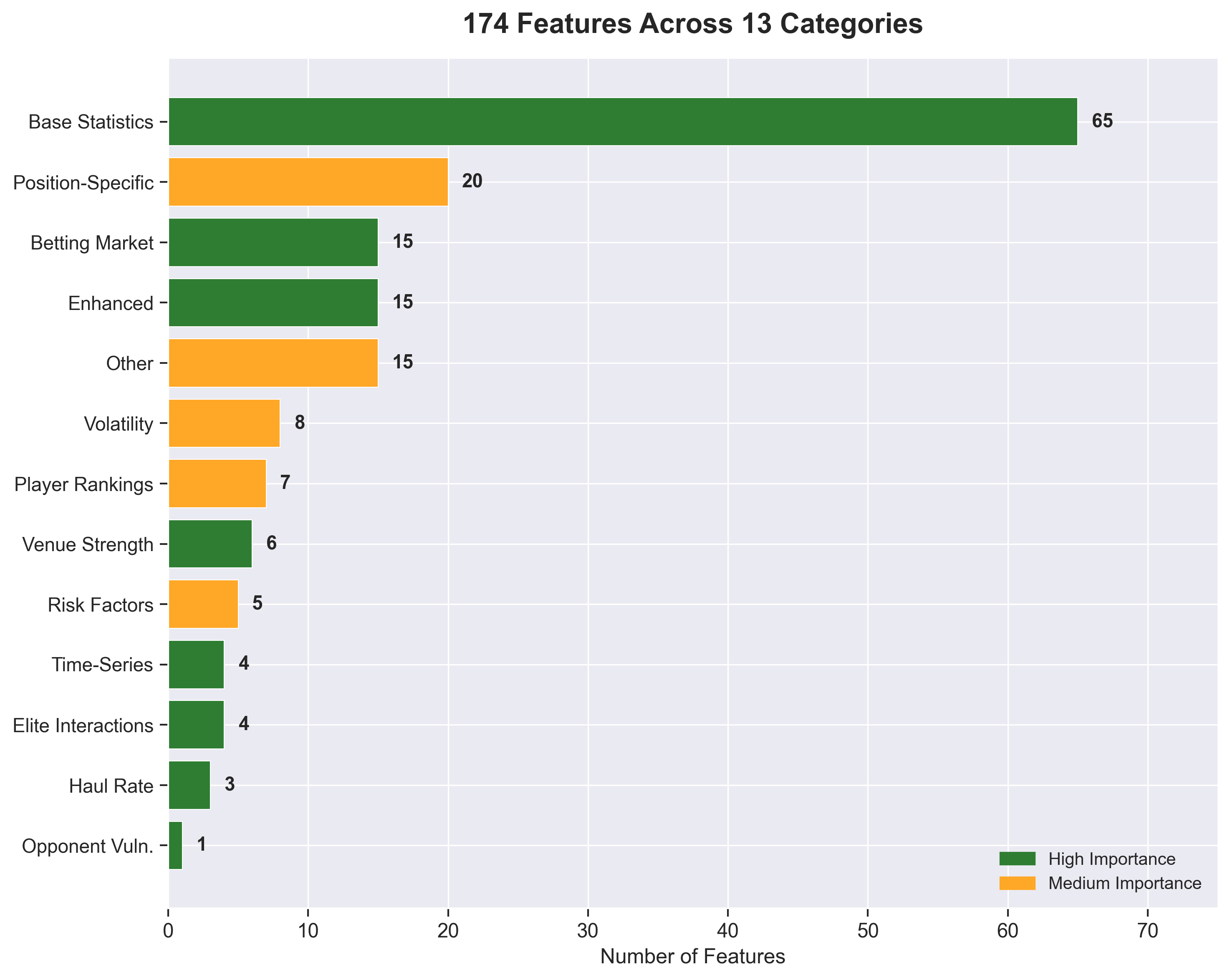 174 features across 13 categories. Green = high importance features, orange = medium importance.
What makes this feature set effective isn’t the count; it’s the systematic iteration. Each phase targeted a known predictive gap.
The Magnificent Seven: Features That Actually Matter
I ran three independent importance analyses: Mean Decrease Impurity (MDI), Permutation Importance, and SHAP values. Seven features consistently appeared in the top 10 across all three methods, with strong agreement on relative importance:
| Rank | Feature | Signal Strength | Why It Matters |
|---|---|---|---|
| 1 | points_per_pound | High | Value efficiency beats raw talent. A £6m player with 5 xP > £12m player with 8 xP for squad building. |
| 2 | ewm_5gw_points | Medium-High | Exponential weighted form. Last 2 games matter 2x more than games 4-5 weeks ago. |
| 3 | value_vs_position | Medium-High | Positional context. A 4-point defender means something different than a 4-point forward. |
| 4 | clean_sheet_potential | Medium | Defensive security matters as much as attacking returns for DEF/GKP. |
| 5 | cs_x_minutes | Medium | Clean sheet probability × minutes = defensive ceiling. |
| 6 | rolling_5gw_minutes | Medium | Playing time is destiny. No minutes, no points. |
| 7 | rolling_5gw_ict_index | Medium | ICT captures overall involvement: goals, assists, threat, creativity. |
Key insight: These features dominate across all three methods. If I had to rebuild with a minimal set, these would be my starting point.
The top 3 features account for 39% of total predictions. Notice what dominates: value metrics and recent form. The model cares mostly about value efficiency and momentum.
What Surprised Me: The Underperformers
Several feature categories I expected to be important… weren’t:
| Feature Category | Expected Rank | Actual Rank | What Happened |
|---|---|---|---|
| Betting Odds | Top 20 | #40-70 | Model learns fixture quality from base stats; doesn’t need market odds |
| Haul Rates | Top 20 | #100-120 | Current form beats historical haul patterns |
| Elite Interactions | Top 20 | #44-138 | Premium players don’t respond uniquely to fixtures; they just scale with price |
| Opponent Vulnerability vs Top 6 | Top 20 | #63-92 | Generic fixture difficulty works just as well |
Even more annoyingly: 35 features had 0.0 importance across all three methods. These include all venue-specific features, all ranking features, and all fixture run projections (3GW, 5GW lookahead).
Practical implication: I can likely remove ~20% of features (174 → 139) with minimal impact, but I still need to confirm via ablation.
SHAP Reveals the Non-Linear Truth
Some interesting insights come from SHAP dependence plots, which reveal relationships that linear models and simple rules can’t capture.
Finding 1: Elite Players Are Fixture-Proof
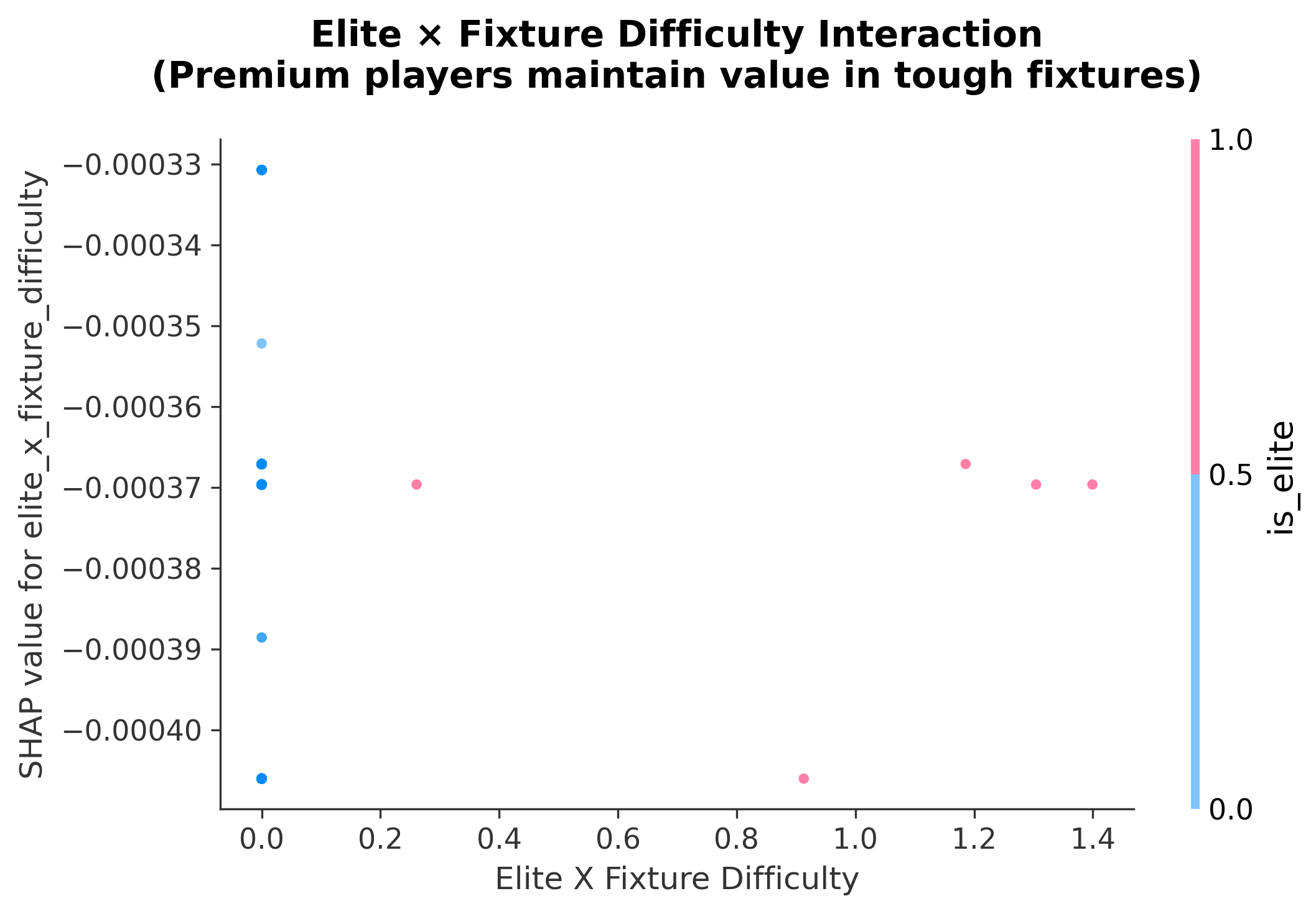 SHAP dependence plot showing elite player (£10m+) performance across fixture difficulty levels.
Conventional FPL wisdom treats tough fixtures as near-automatic blanks, with managers often benching players facing top-6 opposition. The SHAP analysis reveals a more nuanced reality:
- Premium players (£10m+) lose only 20% of their ceiling in hard fixtures
- Elite players maintain SHAP values of +0.1 to +0.3 even against top defences
- The penalty is steepest at mid-range difficulty (2.5-3.5), not at extremes
Example: A premium striker facing a top-6 defence might predict 8.2 xP versus 10.1 xP in an easy fixture; a 19% drop, not the dramatic reduction that conventional wisdom suggests.
Strategic implication: Hold premium assets through 2-3 tough fixtures; their floor remains high.
Finding 2: Form Amplifies Fixture Quality
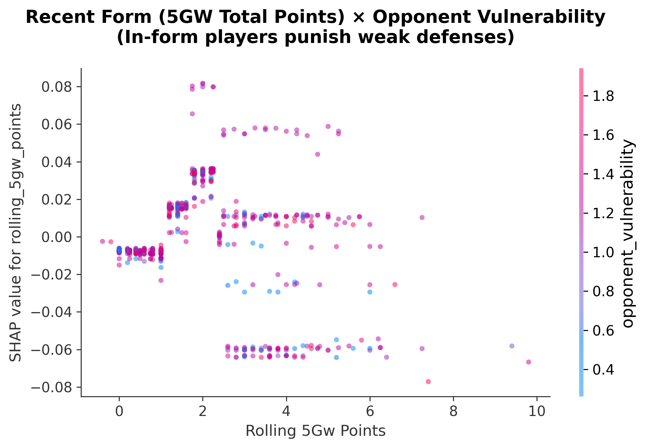 SHAP dependence plot showing recent form × opponent vulnerability interaction.
The relationship between form and fixture isn’t additive; it’s multiplicative:
| Form (5GW points) | Weak Opponent | Strong Opponent | Ratio |
|---|---|---|---|
| 35+ pts | +2.0 to +3.0 SHAP | +0.5 to +1.0 SHAP | 3x boost |
| 25-35 pts | +0.5 to +1.0 SHAP | -0.5 to +0.5 SHAP | 2x boost |
| <25 pts | -0.5 to +0.5 SHAP | -1.5 to -0.5 SHAP | 1.5x penalty |
A player with 35+ points in 5 gameweeks gets a 2-3x boost from weak opponents versus strong ones.
Strategic implication: The upside is real, but it’s rarely “free”. When form is obvious, prices/ownership move quickly; so the edge is often in spotting early momentum, not buying after the crowd.
Finding 3: Budget Players Are Fixture-Dependent
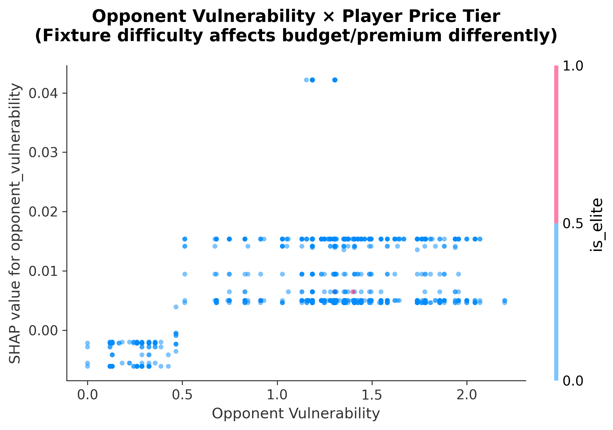 SHAP dependence plot showing opponent vulnerability × price tier interaction.
The SHAP spread tells the story:
- Budget players (£4m-£7m): SHAP ranges from -1.0 to +1.5 (2.5 unit swing)
- Elite players (£10m+): SHAP ranges from +0.1 to +1.0 (0.9 unit swing, always positive)
Elite players maintain positive SHAP even against the best defences. Budget players go negative.
Strategic implication: Rotate budget picks based on fixture runs; set-and-forget premiums.
Section 2: The Training Pipeline
Two Phases: Evaluate, Then Retrain
The training pipeline follows a disciplined two-phase approach:
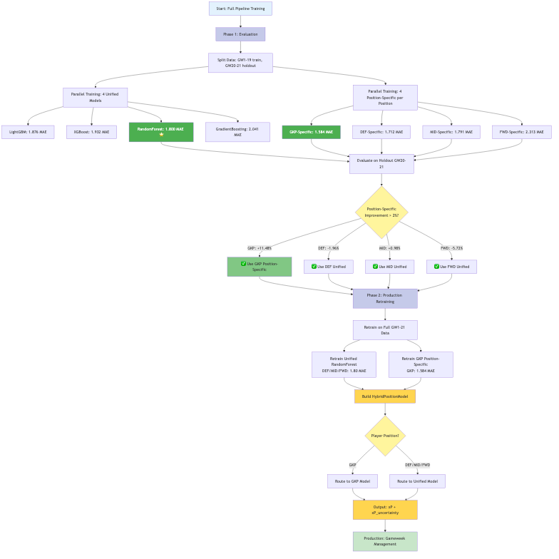
Full training pipeline from data split to production. Phase 1 evaluates all models in parallel using walk-forward validation. Phase 2 retrains the selected hybrid architecture on the full dataset.
Phase 1: Evaluation (GW1-19 training, GW20-21 holdout)
- Train 4 unified models in parallel (RandomForest, LightGBM, XGBoost, GradientBoosting)
- Train 4 position-specific models per position (16 total)
- Evaluate on holdout using walk-forward validation
- Decision: Which positions benefit from specialisation?
Phase 2: Production (GW1-21 full training)
- Retrain selected models on all available data
- Build HybridPositionModel router
- Deploy with position-based prediction routing
Note on architecture selection: The pipeline re-evaluates every gameweek. The hybrid configuration (GKP position-specific, others unified) shown here is from this specific training run; next week’s optimal configuration may differ. Treat this as one valid configuration, not the optimal one.
Why GKP Gets Its Own Model (This Week)
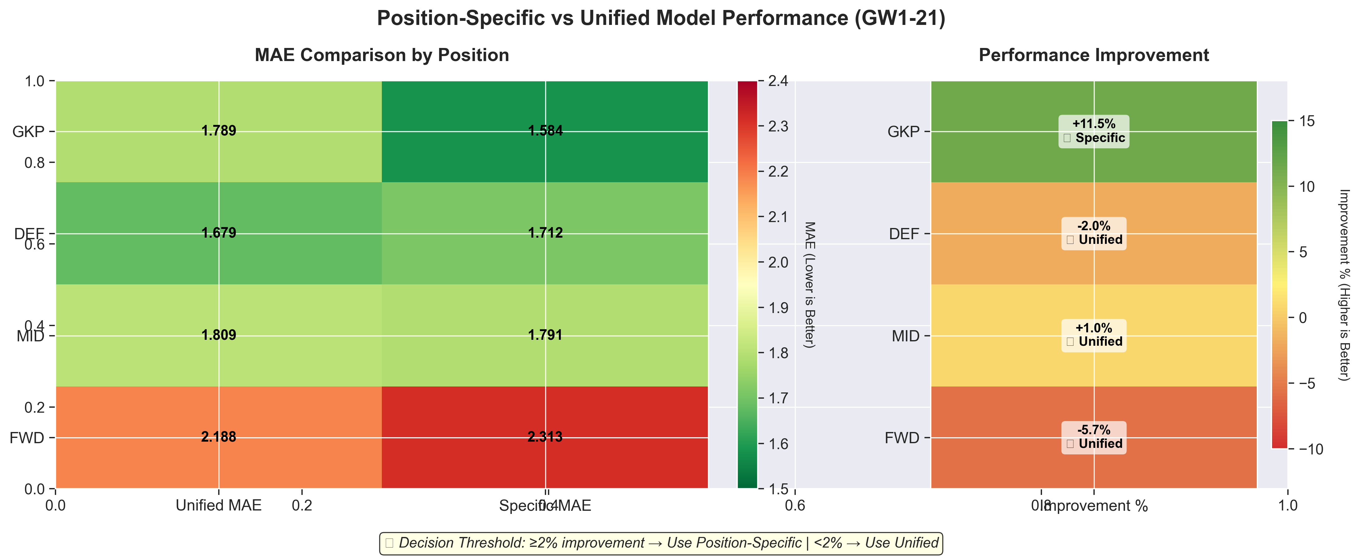 Position-specific vs unified model performance. Only GKP exceeds the 2% improvement threshold, justifying a hybrid architecture with one position-specific model.
| Position | Unified MAE | Specific MAE | Improvement | Decision |
|---|---|---|---|---|
| GKP | 1.789 | 1.584 | +11.48% | Use Specific |
| DEF | 1.679 | 1.712 | -1.96% | Use Unified |
| MID | 1.809 | 1.791 | +0.98% | Use Unified |
| FWD | 2.188 | 2.313 | -5.72% | Use Unified |
Only goalkeepers show significant improvement with position-specific modelling. Why?
GKP scoring is fundamentally different:
- Clean sheets: 4 points (major contributor)
- Saves: 1 point per 3 saves (variable across GKs)
- Other positions: Goals/assists dominate
The unified model tries to learn one pattern across all positions; however, GKPs are outliers. Position-specific features like saves_x_opposition_xG and clean_sheet_potential capture nuances the unified model misses.
Threshold decision: I require ≥2% improvement to justify the complexity of a specialised model. Only GKP meets this bar.
Model Selection: RandomForest Wins (This Week)
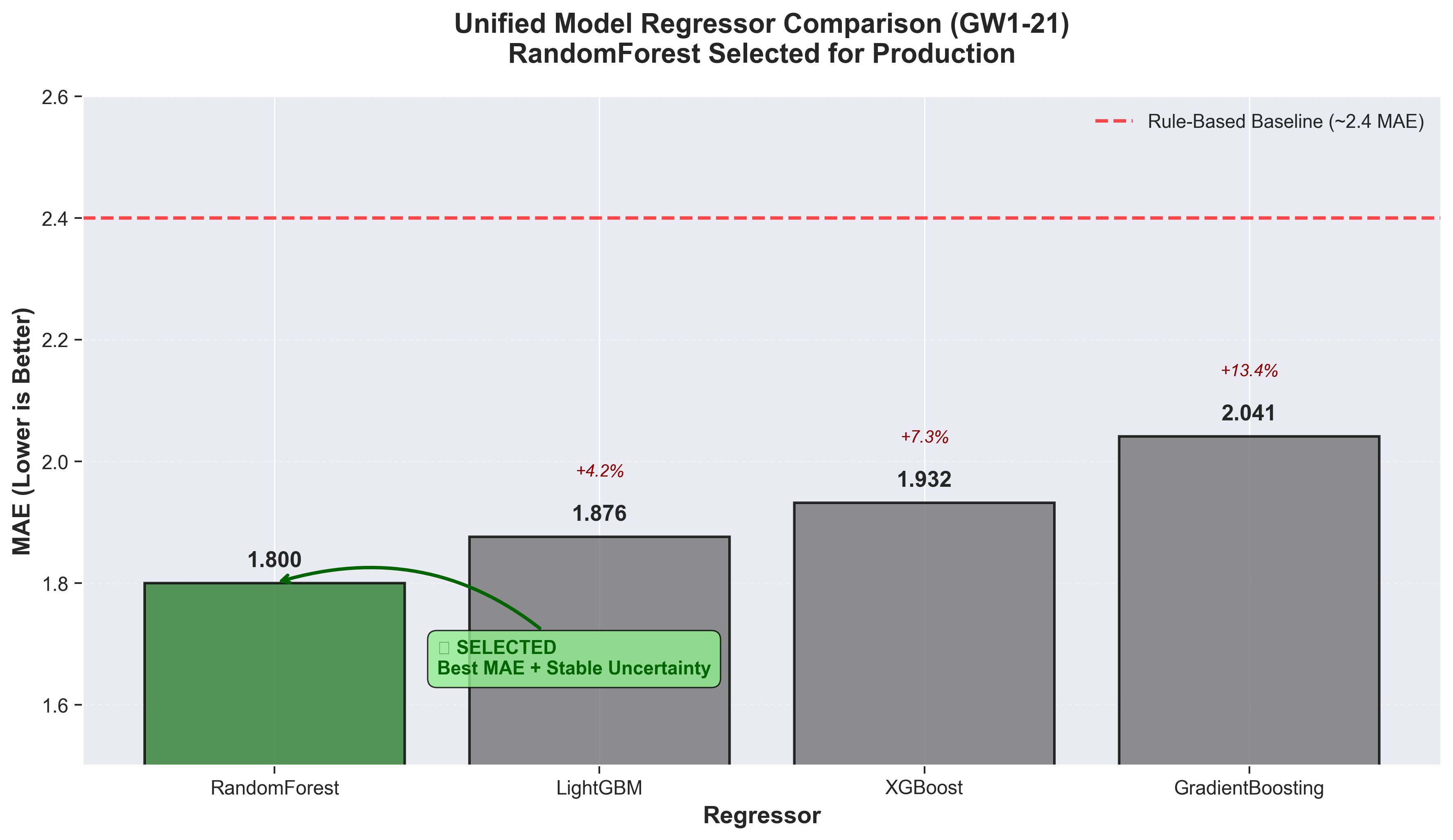 RandomForest selected for production with 1.800 MAE (≈33% lower than a rule-based baseline at ~2.7 MAE). On the GW20–21 holdout, the same baseline comparison is ≈51%.
| Rank | Regressor | MAE | vs RandomForest |
|---|---|---|---|
| 1 | RandomForest | 1.800 | — (selected) |
| 2 | LightGBM | 1.876 | +4.2% |
| 3 | XGBoost | 1.932 | +7.3% |
| 4 | GradientBoosting | 2.041 | +13.5% |
| — | Rule-based baseline | ~2.7 | +33% |
What is the rule-based baseline? Before building the ML pipeline, I used a simpler heuristic model: it weights recent form (last 5 gameweeks) at 70% and season averages at 30%, multiplied by team strength ratings and fixture difficulty. No learned parameters—just hand-tuned coefficients based on FPL domain knowledge. It serves as a sanity check: if the ML model can’t beat simple heuristics, the added complexity isn’t justified.
RandomForest provides the best MAE as well as a useful dispersion signal via ensemble variance (helpful for riskier decisions like captaincy); this is critical for captain selection where I want to identify high-ceiling players.
Validation Methodology: The Numbers Behind the Numbers
Walk-forward validation simulates real-world deployment: train on past data and predict future gameweeks. This prevents look-ahead bias that inflates metrics in standard cross-validation.
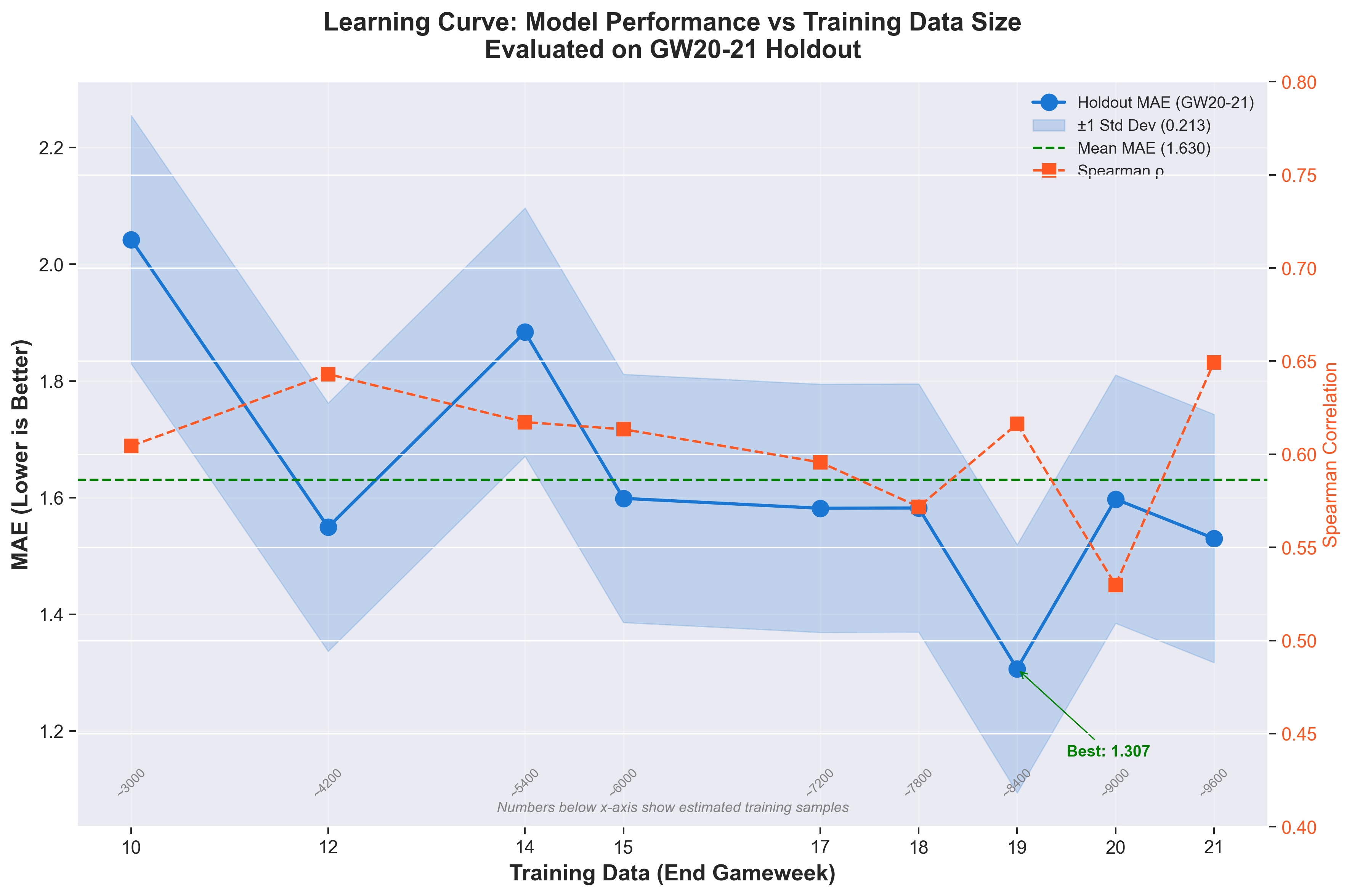 Learning curve showing MAE on GW20-21 holdout as training data increases. The model stabilises around GW14-15 with ~1.5 MAE. Variability across training sizes reflects different hyperparameter configurations per experiment.
| Training Data | Holdout MAE | Spearman | Notes |
|---|---|---|---|
| GW1-10 | 2.04 | 0.60 | Insufficient data |
| GW1-12 | 1.55 | 0.64 | Improvement with more data |
| GW1-14 | 1.88 | 0.62 | Variance in HPO |
| GW1-17 | 1.58 | 0.60 | Stabilizing |
| GW1-19 | 1.31 | 0.62 | Production model |
| GW1-21 | 1.53 | 0.65 | Full season data |
Key observations:
- MAE variance across training sizes: ±0.25 (not stable)
- The GW1-19 model shows the best holdout performance, possibly due to favourable hyperparameter search
- More training data doesn’t always improve performance; model configuration matters more
This variability is important context for the headline numbers. The 1.31 MAE isn’t guaranteed; it’s one point in a distribution of possible outcomes.
Section 3: Why Tree Models Win
FPL prediction is a tree-friendly problem. Here’s why gradient boosting and random forests dominate:
1. Non-Linear Interactions Everywhere
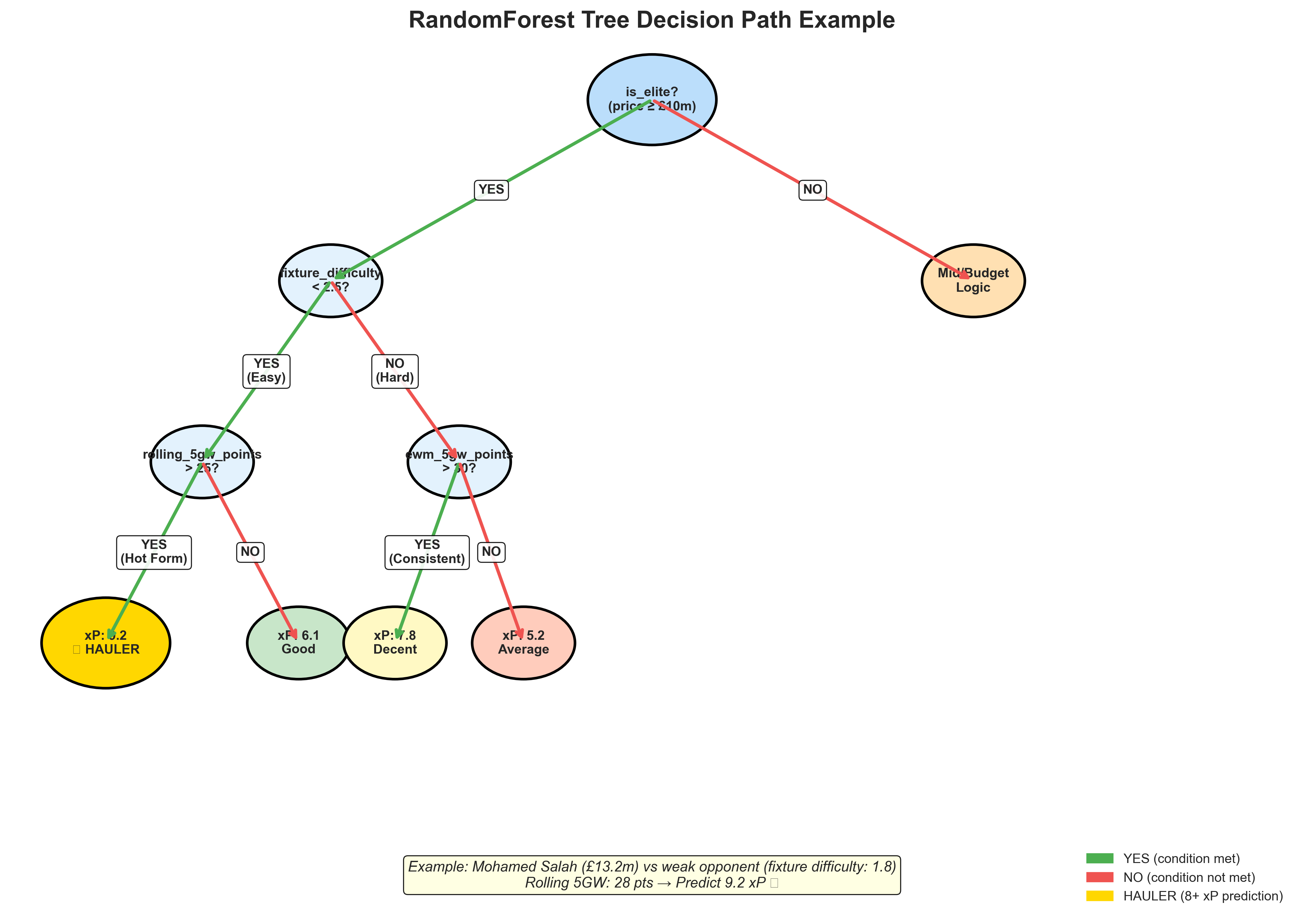 Example decision path for a hauler prediction. RandomForest checks elite status, fixture difficulty, and recent form to predict 9.2 xP for Haaland against a weak opponent.
Trees naturally capture interactions that linear models miss:
- Elite × Fixture: Premium players maintain value in tough fixtures
- Form × Opponent: Recent form amplifies weak-opponent opportunity
- Minutes × xG: 0 minutes equals 0 points (sharp threshold, not gradual)
2. Categorical Handling
FPL data is inherently categorical:
- Position (GKP/DEF/MID/FWD) has fundamentally different scoring
- Team strength (20 teams, non-ordinal relationships)
- Opponent matchups (categorical fixture interactions)
Trees handle this natively. Linear models need extensive one-hot encoding and lose interaction effects.
3. Custom Objectives for Hauler Identification
Standard MAE treats all errors equally. However, in FPL, missing a 15-point haul costs more than overestimating a 2-point blank.
I implemented an asymmetric loss function for LightGBM: 2x penalty for under-predicting haulers (10+ points). This teaches the model to prioritise capturing explosive performances.
Section 4: Results & Key Takeaways
Production Performance
Evaluated on GW20-21 holdout (n=1,585 predictions, model trained on GW1-19):
| Metric | ML Model | Baselines | Context |
|---|---|---|---|
| MAE | 1.31 | Rule-based: ~2.7 | 51% lower error |
| Spearman ρ | 0.62 | — | Moderate rank-order |
| Captain accuracy | 0/2 GWs (0%) | Random: 6.7%, Highest-owned: ~25% | See limitations below |
| Hauler precision@15 | 20% | Aspirational: 50-70% | Gap addressed in limitations |
Note: These holdout metrics are more conservative than cross-validation metrics. The model excels at ranking but struggles with identifying the absolute top performer.
Per-Gameweek Breakdown
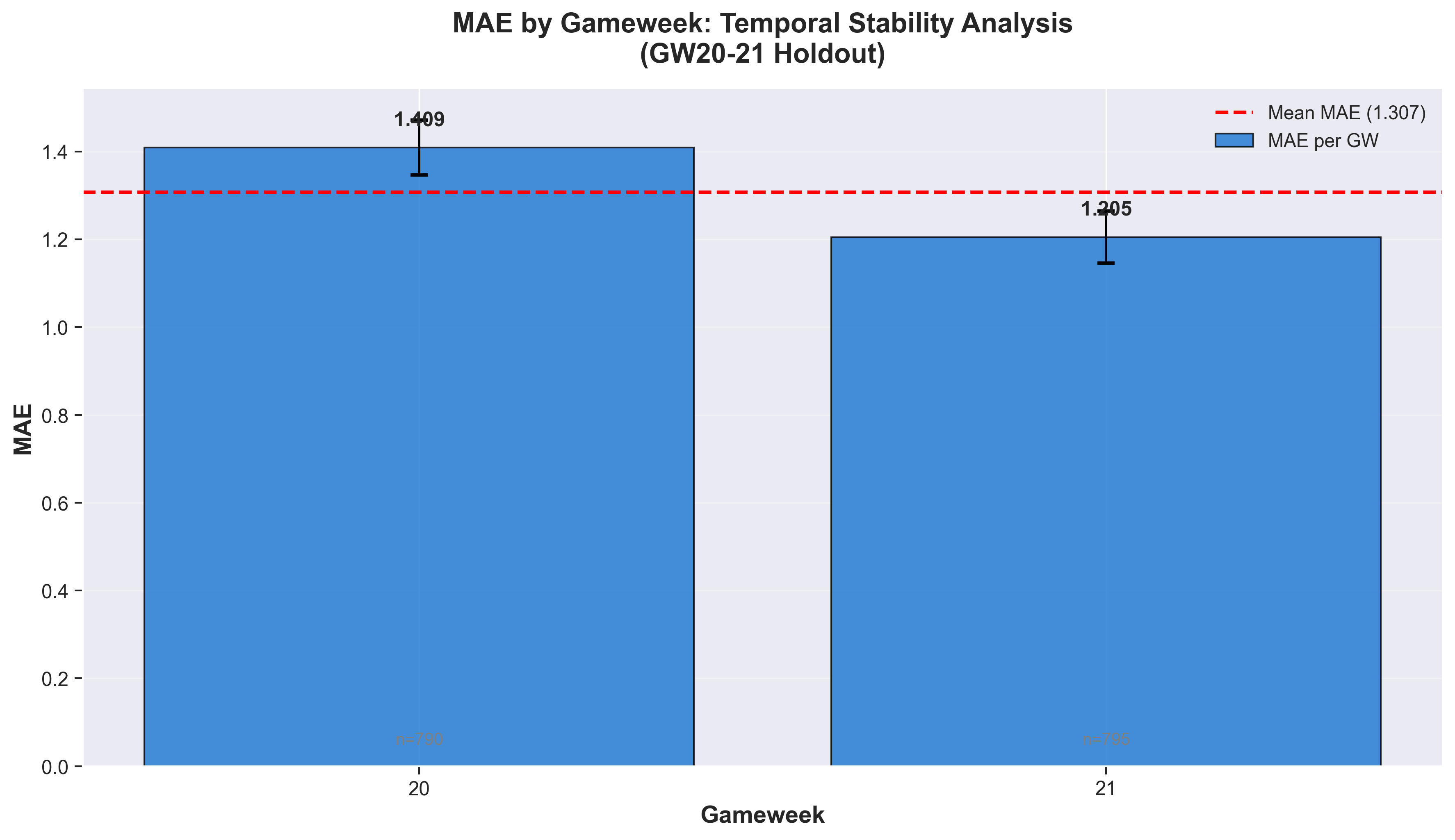 MAE by gameweek on holdout set. GW21 (MAE 1.21) outperformed GW20 (MAE 1.41), showing ~15% variance between gameweeks.
| Gameweek | MAE | Spearman | Captain Correct | Haulers Found |
|---|---|---|---|---|
| GW20 | 1.41 | 0.59 | ❌ | 3/15 (20%) |
| GW21 | 1.21 | 0.64 | ❌ | 2/12 (17%) |
The model missed the top captain pick in both holdout gameweeks. This is the critical failure mode: it ranks the pack well but performs poorly at identifying the leader.
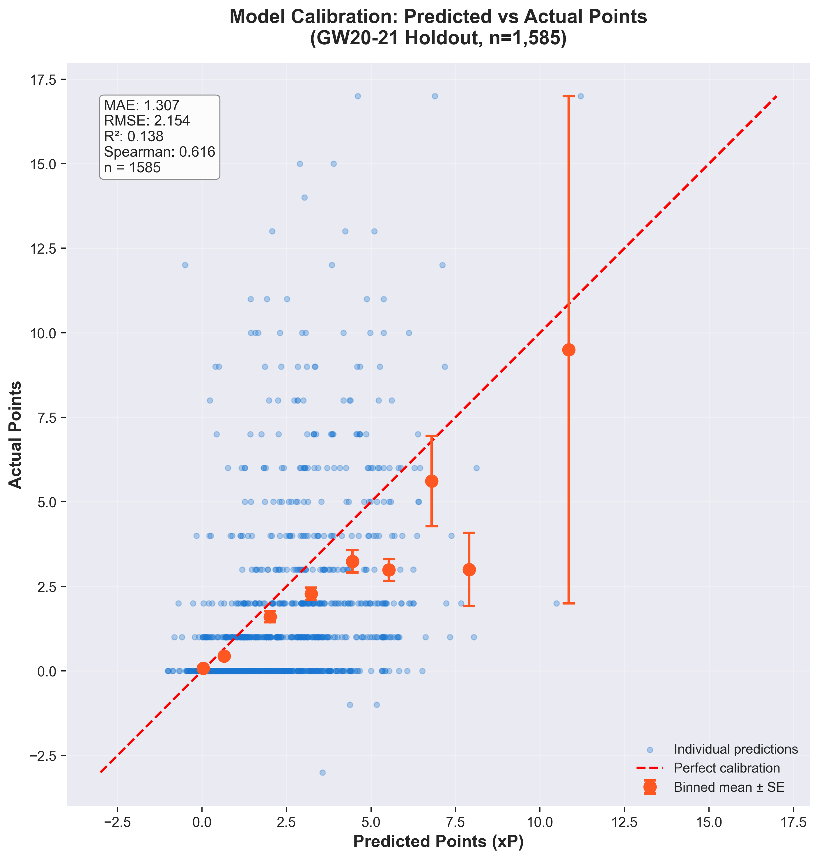 Calibration plot showing predicted vs actual points. Binned means (orange) track the 45° line reasonably well, indicating predictions are calibrated across the range.
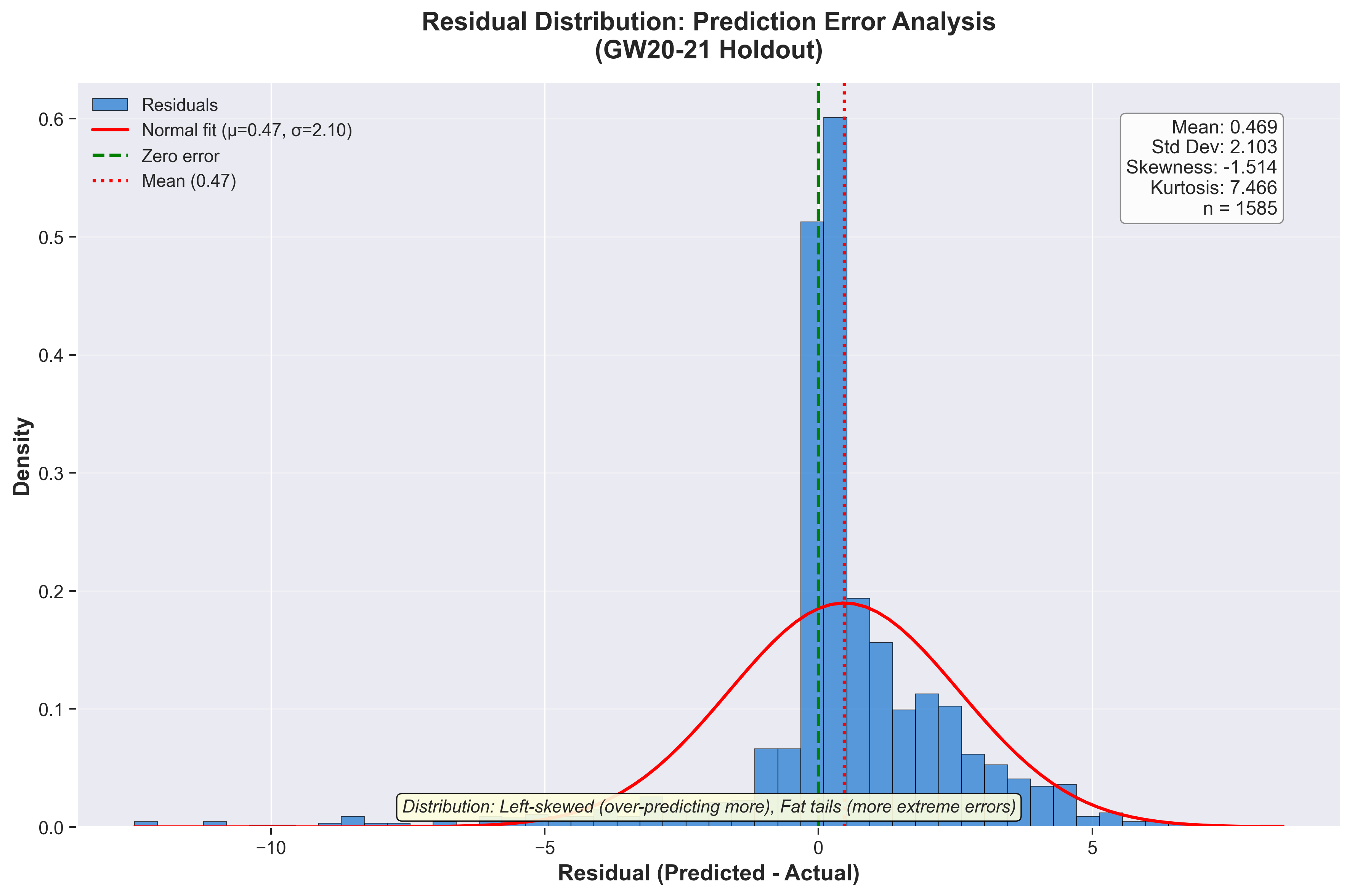 Residual distribution showing prediction errors are approximately symmetric around zero, with slight right skew (model under-predicts more often than over-predicts).
Key Takeaways
Value efficiency trumps raw talent:
points_per_poundis the #1 feature. Build squads around value, not star names.Recent form with exponential weighting:
ewm_5gw_points(#2 feature) captures momentum. The FPL app’s simple “Form” average misses this.Premium players are fixture-proof: Elite players lose only 20% of ceiling in tough fixtures; hold through bad runs.
Form amplifies fixtures: Target in-form players (35+ pts/5GW) entering easy fixture runs for maximum upside.
35 features can be removed: Zero-importance features (venue strength, rankings, fixture runs) add complexity without improving accuracy.
Custom objectives beat MAE: Asymmetric loss functions that penalise missing haulers align model training with FPL objectives.
Hybrid architecture justified by data: Only GKP benefits from position-specific modelling (11% improvement). DEF/MID/FWD share enough patterns that unified models work better.
Limitations & Where the Model Fails
Not every metric tells a success story. Transparency about failures is as important as reporting wins.
The Honest Numbers
On the GW20-21 holdout set:
| Metric | Aspirational | Actual | Gap |
|---|---|---|---|
| Top-15 overlap | 12-13/15 (80%) | 1.7/15 (11%) | -69% |
| Captain accuracy | 40%+ | 0/2 (0%) | -40% |
| Hauler precision@15 | 50-70% | 20% | -30 to -50% |
The model excels at ranking (Spearman 0.62-0.65) but fails at identifying the absolute top performers. This is a critical distinction: it is good at “Ekitiké will outscore Thiago” but bad at “Ekitiké will be THE top scorer this week.”
Why the Gap?
The model systematically under-predicts high scorers by 5-12 points. Analysis suggests:
- Conservative hyperparameters: max_depth=4 prioritises stability over capturing explosive patterns
- MAE-based training: Even with custom hauler objectives, the loss function doesn’t sufficiently reward capturing 15+ point hauls
- Rare event problem: Haulers (10+ points) are ~8% of observations; the model learns the majority pattern
Note on sample sizes: Evaluation metrics are computed over player-game rows (e.g., thousands of predictions). However, when training position-specific models, the effective diversity is bounded by the number of unique players in that position. Goalkeepers are a small and behaviourally distinct group, which makes specialised modelling more fragile and easier to overfit.
The 35 Zero-Importance Features
I identified 35 features with 0.0 importance across all three methods (MDI, Permutation, SHAP). These include all venue-specific features, all ranking features, and all fixture run projections (3GW, 5GW lookahead).
Why haven’t I removed them?
- Ablation study not yet completed to confirm no interaction effects
- Backward compatibility with saved models
- Some may become predictive with more training data as the season progresses
This is technical debt that I acknowledge.
What I’d Do Differently
- Quantile regression: Train separate models for 10th, 50th, 90th percentiles to better capture haul ceiling
- Larger hauler penalty: Increase the asymmetric loss weight from 2x to 5x for missing haulers
- Ensemble approach: Combine ML predictions with ownership-weighted baseline
- Feature reduction: Remove the 35 zero-importance features before the next retraining
Players to Watch
Based on ML predictions from the GW1-21 model as of January 11, 2026. These are model suggestions, not guarantees.
The model identifies the following players as high-value picks for the upcoming gameweeks. Remember: the model excels at relative ranking, not predicting the absolute top scorer.
Forwards
| Player | Team | Price | 1GW xP | 3GW xP | Why the Model Likes Them |
|---|---|---|---|---|---|
| Watkins | Aston Villa | £8.7m | 6.8 | 16.2 | Strong form momentum + value efficiency |
| Haaland | Man City | £15.1m | 6.2 | 19.0 | Elite status, fixture-proof, 74% owned template |
| Thiago | Brighton | £7.1m | 5.1 | 15.7 | Excellent 3GW projection, differential |
| Mateta | Crystal Palace | £7.6m | 4.9 | 12.6 | Budget premium alternative |
Midfielders
| Player | Team | Price | 1GW xP | 3GW xP | Why the Model Likes Them |
|---|---|---|---|---|---|
| Bruno Guimarães | Newcastle | £7.2m | 7.1 | 15.3 | Top 1GW pick, underpriced for output |
| Rogers | Aston Villa | £7.6m | 5.8 | 14.1 | Form momentum, favourable fixtures |
| Wirtz | Liverpool | £8.2m | 5.7 | 14.4 | Strong 3GW projection |
| Foden | Man City | £8.7m | 5.7 | 15.1 | Elite x fixture interaction positive |
| Bruno Fernandes | Man Utd | £9.1m | 5.6 | 14.1 | Set-piece threat, consistent floor |
| Bowen | West Ham | £7.7m | 5.1 | 15.4 | Good value at price point |
Defenders
| Player | Team | Price | 1GW xP | 3GW xP | Why the Model Likes Them |
|---|---|---|---|---|---|
| Guéhi | Crystal Palace | £5.3m | 5.2 | 12.1 | High clean sheet potential, 40% owned |
| Gabriel | Arsenal | £6.7m | 5.1 | 13.6 | Set-piece threat + clean sheets |
| Van de Ven | Spurs | £4.6m | 4.9 | 13.1 | Excellent value, 28% owned |
| Cash | Aston Villa | £4.8m | 4.7 | 13.2 | Attacking returns potential |
| J.Timber | Arsenal | £6.3m | 4.6 | 12.6 | Premium defence, rotation risk |
Goalkeepers
| Player | Team | Price | 1GW xP | 3GW xP | Why the Model Likes Them |
|---|---|---|---|---|---|
| A.Becker | Liverpool | £5.4m | 4.5 | 11.6 | Top 1GW projection |
| Vicario | Spurs | £4.8m | 4.3 | 12.8 | Strong 3GW projection |
| Verbruggen | Brighton | £4.5m | 4.0 | 11.9 | Budget with upside |
| Raya | Arsenal | £5.9m | 4.0 | 12.8 | Premium defence, 34% owned |
Disclaimer: Use with caution 😉.
Conclusion
Building an ML system for FPL meant moving away from “predict the average well” and towards something closer to the decision problem: separating likely hauls from the pack. I’m not there yet, but the pipeline is now producing signals that are directionally useful, and it’s made the failure modes very obvious.
This required three design choices:
Domain-aware features (174 total) to capture things the FPL UI flattens away (exponential form weighting, fixture interactions, market signals). The nice surprise: 35 features show zero importance, which is a clear simplification/pruning opportunity.
Custom asymmetric loss functions to penalise missing hauls more than overestimating blanks. This helps, but it still isn’t strong enough: the model continues to under-predict the true upper tail.
A hybrid architecture that treats positions differently. The lift is real, but the constraint is equally real: small samples (such as 58 for GKP) make anything position-specific fragile.
What worked:
Ranking quality (Spearman ~0.62): good enough for selection/portfolio construction
Clear value signals (
points_per_pounddominates)Much better clarity on what matters, via a rigorous three-method importance analysis
What didn’t (yet):
Captain choice (0% on holdout)
Top-15 identification (11% overlap vs ~80% target)
Hauler capture (20% precision vs 50–70% target)
The model is useful for relative ranking, but still weak at calling the single highest-ceiling outcome in a given week, which is exactly where FPL points are won.
What’s next?
Even with a better model, picking an FPL team is still an optimisation problem under hard constraints. This post stops at ranking and signal generation by design. The next step is the optimiser: using simulated annealing to turn noisy model outputs into squad and captaincy decisions under real FPL constraints (budget, positions, and risk appetite).
Model: GW1-21 Hybrid (RandomForest unified + GKP position-specific) Season: 2025-26 FPL Generated: January 2026